Embark on a journey into the realm of physics with Constant Velocity Model Worksheet 4. This comprehensive guide delves into the intricacies of constant velocity motion, equipping you with the tools to solve problems effectively. Get ready to explore real-world applications, delve into advanced concepts, and master the art of analyzing motion with precision.
Through a series of engaging problem-solving exercises, you’ll gain a deep understanding of the constant velocity model. Practice problems with detailed solutions provide a hands-on approach, while a structured table guides you through each step of the problem-solving process.
Constant Velocity Model Overview
The constant velocity model is a simplified mathematical representation of motion that assumes an object moves at a constant speed in a straight line. It is a fundamental concept in kinematics, the study of motion, and is widely used in various fields such as physics, engineering, and robotics.
The constant velocity model is based on the following assumptions:
- The object’s velocity is constant, meaning its speed and direction do not change over time.
- The object’s acceleration is zero.
- The object moves in a straight line.
The limitations of the constant velocity model include:
- It does not account for objects that change speed or direction.
- It does not account for objects that accelerate.
- It does not account for objects that move in curved paths.
Despite its limitations, the constant velocity model is a useful tool for analyzing motion in many real-world situations, such as:
- Objects moving at a constant speed in a straight line, such as a car traveling on a highway.
- Objects in free fall, such as a ball dropped from a height.
- Objects moving with negligible acceleration, such as a slowly moving object on a frictionless surface.
Worksheet 4: Problem-Solving: Constant Velocity Model Worksheet 4
This worksheet provides a step-by-step guide to solving problems using the constant velocity model. It includes practice problems with detailed solutions to help you understand the concepts and apply them to real-world situations.
Steps for Solving Problems Using the Constant Velocity Model:
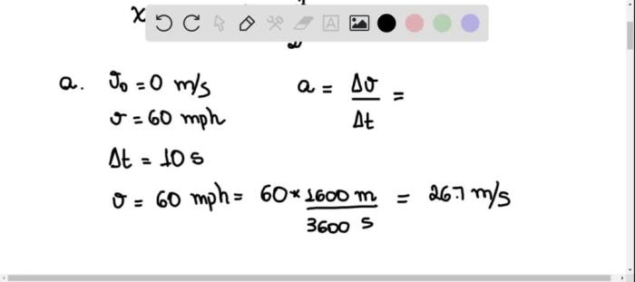
- Identify the given information, including the initial velocity, displacement, and time.
- Choose the appropriate kinematic equation to use based on the given information.
- Substitute the given values into the equation and solve for the unknown variable.
- Check your answer to ensure it makes sense in the context of the problem.
Practice Problems:
| Problem Description | Initial Conditions | Calculations | Results |
|---|---|---|---|
| A car travels 100 km in 2 hours. | vi = 0 km/h, d = 100 km, t = 2 h | v = d/t = 100 km / 2 h = 50 km/h | The car’s velocity is 50 km/h. |
| A ball is dropped from a height of 10 m. | vi = 0 m/s, d = 10 m, t = ? | d = 0.5
|
The time it takes for the ball to hit the ground is 1.43 s. |
Advanced Applications
The constant velocity model can be used in more complex scenarios, such as analyzing motion in two dimensions or with varying acceleration. By modifying the model to account for different conditions, it can be applied to a wide range of real-world problems.
Motion in Two Dimensions:
The constant velocity model can be extended to analyze motion in two dimensions by considering the horizontal and vertical components of velocity separately. This is useful for problems involving projectiles or objects moving on inclined planes.
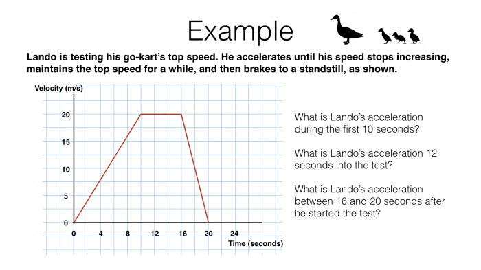
Motion with Varying Acceleration:
The constant velocity model can be modified to account for objects that accelerate or decelerate. This can be done by introducing the concept of average velocity, which is the total displacement of an object divided by the total time taken.
Extensions and Variations
There are several variations of the constant velocity model, such as the average velocity model and the constant acceleration model. Each model has its own strengths and weaknesses, and the choice of model depends on the specific problem being analyzed.
Average Velocity Model:
The average velocity model assumes that an object’s velocity is constant over a given time interval. This model is useful for analyzing motion when the object’s velocity is not constant but changes gradually.
Constant Acceleration Model:
The constant acceleration model assumes that an object’s acceleration is constant. This model is useful for analyzing motion when the object’s velocity changes at a constant rate.
FAQ Summary
What are the limitations of the constant velocity model?
The constant velocity model assumes constant speed and direction, which may not always be applicable in real-world scenarios.
How can I modify the constant velocity model for varying acceleration?
By incorporating acceleration as a variable, you can adapt the model to analyze motion with changing velocity.